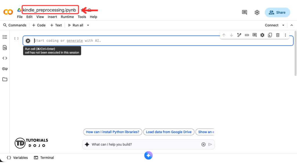
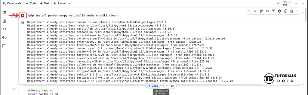
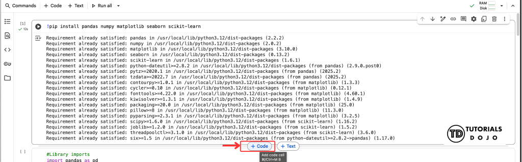
Before machine learning (ML) models can generate predictions or insights, the raw data must first be cleaned, organized, and transformed into a suitable format for the model. This process is known as data preprocessing. It is the foundation of every successful ML project. It ensures that the model learns from high-quality, consistent, and well-structured input rather than noisy, incomplete, or biased information. In this hands-on guide, we’ll walk through how to transform a raw Kindle eBook dataset from Kaggle into machine learning-ready data using Google Colab, a free cloud-based environment that allows you to write and execute Python code directly in your browser. Through a series of step-by-step demonstrations, you’ll learn how to inspect, clean, and engineer features that will later improve model accuracy and interpretability. Data preprocessing is where most of the real work and real impact happen. In fact, many data scientists spend up to 80% of their project time cleaning and preparing data. By mastering these techniques, you gain control over the quality of your models and ensure that your results reflect genuine patterns rather than artifacts of messy data. By the end of this guide, you’ll understand: Whether you’re a beginner exploring data science or an intermediate practitioner looking to refine your workflow, this tutorial will give you a practical foundation for turning raw data into reliable, ML-ready insights. Let’s first identify the machine learning problem we are trying to solve before jumping into data preprocessing. It’s essential to understand the problem you are trying to solve. Data preprocessing is not a one-size-fits-all process. The steps you take depend heavily on your project’s objectives, the nature of your data, and the insights you hope to uncover. In this tutorial, we’re working with a Kindle eBook dataset that you can download by clicking the link bellow. To make this data useful for machine learning, we first need to clarify our end goal. In this case, our goal is to preprocess the data to handle a binary classification model that classifies whether a Kindle eBook is likely to become a bestseller or not. By clearly defining the task as a binary classification problem (bestseller vs. non-bestseller), we can: By taking the time to define the problem first, you avoid unnecessary work and ensure that your preprocessing pipeline aligns directly with your modeling goals. To preprocess and analyze our dataset efficiently, we’ll use Google Colab. It provides preconfigured access to common Python data science libraries and GPU/TPU acceleration, making it an ideal tool for beginners and professionals alike. You can access Colab directly through your browser at colab.research.google.com. If you have a Google account, you can access it via Google Drive → New → More → Google Colaboratory. Once opened, create a new notebook by clicking this button. Next, rename it with ‘kindle_processing.ipynb’. Although Colab comes with most common libraries preinstalled, it’s good practice to confirm and install any missing ones. Paste this code in a cell to check if any of the preinstalled libraries are missing. To run the code, click the play button on the upper left of the cell. The code will then execute and will display the output if there is any logs or print statements. To add a new code cell, you need to hover under the cell and two buttons will appear. Clicking on the ‘+ Code’ button will add a new cell bellow it. Next is to import the libraries we’ll use throughout this tutorial: Now, let’s explore the dataset and verify that Colab successfully loaded it. Understanding the dataset is a crucial first step before any preprocessing or modeling work. By examining its structure, data types, and content, you gain insights into how the data is organized, what kinds of values it contains, and where potential issues—such as missing values, duplicates, or inconsistent formats—might occur. By addressing missing data early, we reduce the risk of training a model on incomplete or misleading information. In reference to the code that displayed missing data in the previous section, we will now address the columns with missing values using the following approach: This code replaces the missing We drop rows with missing Finally, let’s confirm that no missing values remain: Before building our model, it’s important to identify and remove these non-essential features. Generally, we consider dropping a column if it meets one or more of the following criteria: Let’s apply this to our Kindle eBook Dataset. In this code, we remove columns such as To confirm the dataset structure after dropping these columns, we can recheck the shape and column names: After dropping irrelevant columns, we can now engineer features that help our model identify patterns more effectively and generate more accurate predictions. Feature engineering is often considered the “art” of machine learning because the quality of features often has a greater impact on model performance than the choice of algorithm or hyperparameter tuning. It involves transforming raw data into meaningful variables during data preprocessing that better represent the underlying problem, improving a model’s ability to learn and generalize to unseen data. Feature engineering also improves model interpretability by creating clearer, more meaningful inputs instead of relying on raw, unprocessed data. Some benefits of feature engineering are the following: In this step, we will use our domain knowledge to creat new, highly informative variables from existing ones. In this code, we convert the This code calculates the length of the Next code will calculate the interaction of Now let’s display the dataset after we engineered new features. It is essential evaluate how a machine learning model perform on unseed data. This is achieved by splitting the dataset into two parts: a training set and a test set. The training set is used to teach the model the patterns and relationships within the data, while the test set is kept aside to evaluate the model’s performance on data it has never seen before. This ensures the model’s results are generizable nad not just memorized from the training data, a problem known as overfitting. Splitting the dataset allows for an unbiased assessment of the model’s accuracy, precision, and other metrics. A common split ration is 80% for training and 20% for testing, though this may vary depending on dataset size and complexity. For this guide, we will split our Kindle eBook data into 80% traing set and 20% test set: This code will set the Now this code will split our dataset into 80% train set and 20% test set. The random state parameter ensures reproducibility of results and stratify parameter maintain class distribution between train and test sets. Let’s now display the size of train and test sets. By splitting the data at this stage, we ensure that all subsequent preprocessing steps, such as encoding or scaling, are applied properly using only the training data. This prevents data leakage and ensuring fair evaluation during model testing. In machine learning, data preprocessing is often the most time-consuming part of the workflow. You can apply transformations one step at a time, but this ad-hoc approach can get messy. It also increases the chance of errors and makes the process harder to reproduce, especially when working with datasets that include numerical, categorical, and boolean features. A preprocessing pipeline provides a structured framework to handle all transformations consistently. Using tools like Scikit-learn’s Pipeline and ColumnTransformer, we can define exactly how each feature type should be processed, for example: Benefits of a preprocessing pipeline include: Most machine learning algorithms work with numerical data. However, many real-world datasets. like the Kindle eBook dataset we are using, contain categorical variables, such as Encoding categorical data is a critical preprocessing step because models interpret numeric values mathematically. Without encoding, algorithms cannot compute relationships or similarities between text-based categories. Why encoding is important: There are several techniques for converting categorical data into numerical form. The choice of method depends on the number and type of categories present. In this guide, One-Hot Encoding is used for nominal features like After encoding, the next step is scaling the numerical features using techniques like StandardScaler. Scaling standardizes the range of continuous variables, ensuring that features with larger numeric values (such as Why scaling is important: Together, encoding and scaling form a foundational stage in the data preprocessing pipeline, ensuring that all input features are consistent, comparable, and optimized for model training. First, let’s identify the data types of the columns in our dataset. This code will set a separate list based on the data type of the column. Next, we will transform the columns. This code creates a ColumnTransformer, a tool from Scikit-learn that applies different preprocessing steps to specific columns. In this case, it uses one-hot encoding for categorical features and standard scaling for numerical variables. These transformations are combined into a single, organized pipeline for easier processing. After the data is transformed, we will now apply these changes to our train set using this code. Make sure to use Now let’s display the shape of transformed data. Preprocessing is the foundation of any machine learning workflow. In this tutorial, we explored the Kindle eBook dataset and prepared it for modeling by: handling missing values, dropping irrelevant columns, engineering new features, encoding categorical variables, scaling numerical features, and building a reproducible pipeline. Proper preprocessing ensures clean, consistent, and numerical data, prevents data leakage, improves model performance, and makes workflows reproducible and maintainable. Investing time in preprocessing sets the stage for accurate and reliable machine learning models. With a clean, preprocessed dataset, the next step is to train and evaluate machine learning models. You can start with algorithms like Logistic Regression, Random Forest, or Gradient Boosting to predict whether a Kindle eBook will become a bestseller. Other possibilities include:
Identify the Problem
Google Colab Setup


!pip install pandas numpy matplotlib seaborn scikit-learn
import pandas as pd
import matplotlib.pyplot as plt
from sklearn.model_selection import train_test_split
from sklearn.preprocessing import StandardScaler, OneHotEncoder
from sklearn.compose import ColumnTransformer
from sklearn.pipeline import Pipeline
from google.colab import files
from imblearn.under_sampling import RandomUnderSampler
from sklearn.model_selection import train_test_split
from collections import Counter
import seaborn as sns
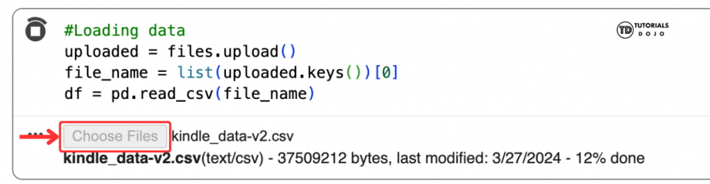
uploaded = files.upload()
file_name = list(uploaded.keys())[0]
df = pd.read_csv(file_name)
Understanding the Dataset
# Display the shape of the dataset
print("Dataset Shape:")
print(df.shape)

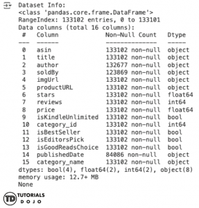
# Display concise summary of the DataFrame
print("Dataset Info:")
print(df.info())
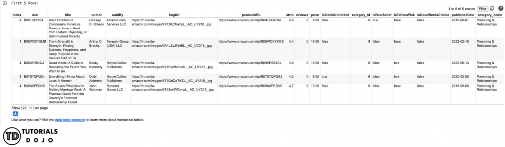
# Display the first few rows
print("First 5 Rows:")
display(df.head())
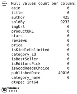
author, soldBy, and publishedDate have null values. We’ll need this later when handling missing data.
# Check for null values and display the count per column
print(df.isnull().sum())
Handling Missing Data
author and soldBy entries with the value 'Unknown'. Doing this ensures that all text data remains complete and can be properly processed later during encoding and scaling steps.
# Fill missing values
# For 'author' and 'soldBy', you could fill with a placeholder like 'Unknown'
df['author'].fillna('Unknown', inplace=True)
df['soldBy'].fillna('Unknown', inplace=True)
publishedDate values because the publication date is a key feature that cannot be accurately imputed without introducing bias or incorrect information. Since the number of missing entries is relatively small, dropping these rows is a safer option that preserves data quality.
# For 'publishedDate', convert to datetime and then drop rows with NaT (missing) values
df['publishedDate'] = pd.to_datetime(df['publishedDate'], errors='coerce')
df.dropna(subset=['publishedDate'], inplace=True)
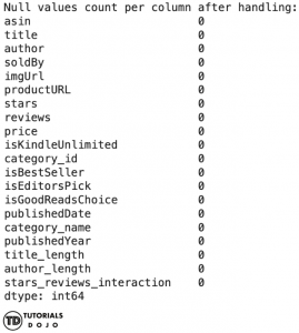
print("nNull values count per column after handling:")
print(df.isnull().sum())
print("nDataset Info:")
print(df.info())
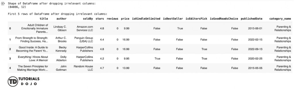
Dropping Irrelevant Columns
url, image, and asin because they act as identifiers or metadata that don’t contribute to predicting whether a book will become a bestseller. By doing this, we simplify the dataset, reduce noise, and make the preprocessing pipeline more efficient. From this stage onward, the df_cleaned variable will serve as our primary dataset, replacing the original df variable for all subsequent steps.
# Columns identified as irrelevant for predicting bestseller status
irrelevant_columns = ['asin', 'imgUrl', 'productURL', 'category_id']
# Drop the specified columns from the DataFrame
df_cleaned = df.drop(columns=irrelevant_columns)
print("Shape of DataFrame after dropping irrelevant columns:")
print(df_cleaned.shape)
print("nFirst 5 rows of DataFrame after dropping irrelevant columns:")
display(df_cleaned.head())
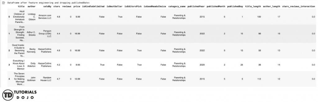
Feature Engineering
publishedDate column into a datetime type so we can extract the day, month, and year into a separate column. We drop the original publishedDate column to avoid redundancy.
# Convert 'publishedDate' to datetime if it's not already
df_cleaned['publishedDate'] = pd.to_datetime(df['publishedDate'], errors='coerce')
# Extract year, month, and day from 'publishedDate'
df_cleaned['publishedYear'] = df['publishedDate'].dt.year
df_cleaned['publishedMonth'] = df['publishedDate'].dt.month
df_cleaned['publishedDay'] = df['publishedDate'].dt.day
# Drop the original 'publishedDate' column as features have been extracted
df_cleaned = df.drop(columns=['publishedDate'])
title and author strings. These features provide simple but useful measures of a book’s characteristics. For instance, title length may serve as a proxy for genre or marketing style, while author length can hint at collaborations or brand recognition — subtle signals the model can learn from.
# Calculate length of 'title' and 'author'
df_cleaned['title_length'] = df['title'].apply(lambda x: len(x) if isinstance(x, str) else 0)
df_cleaned['author_length'] = df['author'].apply(lambda x: len(x) if isinstance(x, str) else 0)
stars and reviews. Multiplying them together gives a combined score that is a much stronger indicator of a book’s true market reception than either factor alone. This allows the model to differentiate between a book with 5 stars and 10 reviews versus one with 4.5 stars and 10,000 reviews.
# Create an interaction term between 'stars' and 'reviews'
df_cleaned['stars_reviews_interaction'] = df_cleaned['stars'] * df_cleaned['reviews']
print("DataFrame after feature engineering and dropping publishedDate:")
display(df_cleaned.head())
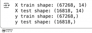
Train & Test Split
isBestSeller column as our taget variable or the ‘y’. We drop the target variable in our ‘X’ or the dataset and set it into a new dataset. Notice that we also droped the title and author columns since we have already feature engineered them into author_length and title_length, this will reduce the noise in our data.
# If column exists, set target properly
target_col = 'isBestSeller'
# Features (X) and Target (y)
X = df_cleaned.drop(columns=['title', 'author', target_col])
y = df[target_col]
# Train-test split
X_train, X_test, y_train, y_test = train_test_split(X, y, test_size=0.2, random_state=42, stratify=y)
# Shape of train-test X
print("X train shape:", X_train.shape)
print("X test shape:", X_test.shape)
#Shape of train-test y
print("y train shape:", y_train.shape)
print("y test shape:", y_test.shape)
Preprocessing Pipeline

Encoding
author, soldBy, or category, which represent text labels rather than numbers. To make these values usable for model training, we need to encode them into numerical form.
soldBy and category_name, while Boolean variables (e.g., isKindleUnlimited) were retained as binary 0/1 values.Scaling
reviews or price) do not dominate smaller-scaled ones (like stars). This step is especially important for distance-based algorithms or models sensitive to feature magnitude.
# Identify columns by type
categorical_cols = ['soldBy', 'category_name']
boolean_cols = ['isKindleUnlimited', 'isEditorsPick', 'isGoodReadsChoice']
numeric_cols = [
'stars', 'reviews', 'price',
'publishedYear', 'publishedMonth', 'publishedDay',
'title_length', 'author_length', 'stars_reviews_interaction'
]
# Define preprocessing for different column types
preprocessor = ColumnTransformer(
    transformers=[
        ('cat', OneHotEncoder(handle_unknown='ignore', drop='first'), categorical_cols), # Encode categorical
        ('num', StandardScaler(), numeric_cols), # Scale numeric
        ('bool', 'passthrough', boolean_cols) # Keep booleans as is (0/1)
    ],
    remainder='drop' # Drop any columns not listed above
)
fit_transform() only on the training set to avoid data leakage.
#Full pipeline (preprocessing only, model can be attached later)
pipeline = Pipeline(steps=[('preprocessor', preprocessor)])
# Fit the pipeline on training data
X_train_encoded = pipeline.fit_transform(X_train)
X_test_encoded = pipeline.transform(X_test)
print("Processed train shape:", X_train_encoded.shape)
print("Processed test shape:", X_test_encoded.shape)
![]()
Conlusion
What’s next?
🔥 $0.99 NEW Study Guide eBook – Claude Certified Associate – Foundations CCAO-F

Turn Your Team Into Cloud-Ready Professionals Today

Learn AWS with our PlayCloud Hands-On Labs

$2.99 AWS and Azure Exam Study Guide eBooks

New Claude Certified Architect Foundations CCA-F

Learn GCP By Doing! Try Our GCP PlayCloud

Learn Azure with our Azure PlayCloud

FREE AI and AWS Digital Courses

FREE AWS, Azure, GCP Practice Test Samplers


Subscribe to our YouTube Channel

Follow Us On Linkedin