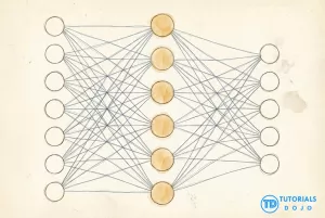
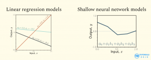
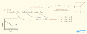
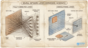
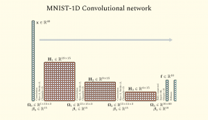
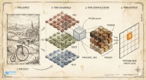
In the age of artificial intelligence, it is common to meet the term neural network, seeing diagrams of neurons connecting to other neurons, programmers training models, and so on. Here, we will discuss how neural networks are similar to plain mathematical functions (models), how they build upon traditional linear regression, and their application to visualize images with convolutional neural networks.

The usual pedagogy for learning neural networks begins with the iconic diagram: columns of circles (“neurons“) connecting to other circles across multiple layers, passing information from input to output. But what is this diagram trying to capture? And what really is a neural network?

Modeling problem

Neural networks are similar to linear regression. Given input data, the linear model fits it, adjusting its slope and intercepts, to find the best-fitting line that predicts the output. Neural networks are similar. It takes inputs, fits a model, and produces output predictions.

The network is often described as a “black box“, where, after training and finding the optimal parameters or weights (adjustable knobs), the model tries to generalize and form predictions that match the real world closely.

The core difference is that neural networks handle much more complex relationships. The diagram simplifies the model to its core: linear regression, which uses straight lines to make predictions. Recognizing this helps us see why adding non-linearity is essential for modeling complex data patterns.

If we look at the simplest possible connection in a network—one input connecting to one output—we are looking at linear regression.

In linear regression, the weights (slope) and biases (additive constants) shift and transform the equation of the line. Given roughly linear data, it fits a straight line, then generalizes and makes predictions. However, linear regression is inherently linear: relationships are straight. But real-world phenomena can be complex and influenced by many variables.

To model the real world, we need to bend the line. Neural networks introduce non-linearity, together with a more complex composition of functions to form the whole model.

The neuron and the formation of a hinge

In biology, a neuron receives signals and decides whether to “fire.” In our mathematical map, we simulate this decision using a non-linear activation function.

In the diagram what composes it is a two-step calculation:

1. Weighted Sum: First, it gathers all incoming signals (arrows), multiplies them by their weights, and adds them up. This is still linear.
2. Activation: Then, it applies a rule to that sum. A common rule is the ReLU (Rectified Linear Unit), which asks a simple question: “Is the value positive? If yes, keep it. If no, turn it off (set to zero).”

This simple operation transforms our straight line into a hinge shape. It creates a corner. This is the crucial spark of complexity: by introducing this non-linearity, we allow the function to change direction.

This switch from linear to non-linear is the core difference between neural networks and linear models. No matter how you compose, multiply, and combine linear functions, the resulting model will still always be linear.

Neural network models introduce the capability to model complex relationships. After all, not all phenomena can be modelled by a single straight line. But in the end, it’s just a model, a mathematical function, which takes in input and returns an output. 

Sculpting the function

A single hinge isn’t very expressive. But what if we had a whole layer of them? What if after computing the inputs and applying an activation function to introduce non-linearity, therby producing a resulting neuron, we further repeat this process where these neurons become the next set of inputs? This is what layers are in neural networks.

A “layer” in the diagram represents a group of these neurons operating in parallel. Since each neuron has its own unique weights, each one creates a hinge at a different location and with a distinct slope.

When the network combines these neurons to produce an output, it is mathematically adding these different hinge shapes together. By summing up enough hinges, we can construct valleys, peaks, and plateaus. We are sculpting a mathematical surface to fit our data.

This introduces the idea of stacking layers to increase model complexity. Each layer builds on the previous one, creating a hierarchy that enables the network to learn increasingly abstract features from raw data.

It creates a hierarchy of composition. The first layer might combine raw inputs to create simple edges (hinges). The second layer combines those edges to create shapes (corners, curves). The third layer combines shapes to form objects.

When you look at a deep neural network diagram, you are looking at an assembly line of functions. You are not just passing data from left to right; you are building increasingly complex computations to handle the complicated behaviour of what the model is trying to predict.

Like linear regression, neural networks are just models that take in inputs and make predictions, but with more capability than just straight lines.

Convolutional neural network

Now that we have a deeper understanding of neural networks. We now jump into a type of neural network highly relevant in the field of images.

The same thinking applies. A convolutional neural network is still a mathematical function that takes in inputs Χ. Undergoing a series of computations and the composition of other functions (arrows, neurons, and layers). By the end, all those computations produce the output Y: the model’s prediction.

If we return to our fundamental premise—that the diagram is just a map of a mathematical function—the “fully connected” network (where every input touches every neuron) reveals a glaring inefficiency when applied to images.

Consider the sheer scale of the arithmetic. A standard image might contain millions of pixels. In a fully connected scheme, a single neuron in the first hidden layer would require a unique weight for every single one of those pixels. That is a mathematical expression with millions of terms to compute one number. If you want a layer with a thousand neurons, you are suddenly managing billions of unique parameters.

In a convolutional layer (right), the connections are sparse and structured.

This isn’t just computationally expensive; it’s statistically brittle. The model becomes a rote memorizer, struggling to generalize. Convolutional Neural Networks (CNNs) solve this by imposing a strict mathematical constraint on the function: parameter sharing.

In the diagram, a convolutional layer often looks like a solid block or a stack of panels. But if we peel back the visualization to the underlying math, we see a dramatic simplification. Instead of a massive unique equation for every neuron, the CNN defines a small, reusable sub-function—often called a kernel or filter.

Stacking the Functions (Channels)

Of course, a single 3 x 3 filter is too simple to understand a complex image. It can perhaps detect vertical lines, but what about horizontal lines, color gradients, or textures?

This is where the concept of channels (or feature maps) enters the equation. In the diagrams, you often see the block’s “depth” increase as the network deepens. This depth represents the number of distinct kernels operating in parallel.

In the following MNIST-1D model, we see how there are multiple channels (columns) which represents how many times the filter is reapplied.

(MNIST-1D Convolutional neural network diagram from Understanding Deep learning (2025) Simon J.D. Prince)

Mathematically, this means we aren’t running just one sliding window function; we are running 64, or 128, or 512 of them simultaneously. Each kernel has its own unique set of weights—one looking for edges, another for color shifts, another for corners. When we stack the outputs of these scans together, we get a multi-dimensional array where every “slice” is a map of where a specific feature was found.

Therefore, a “neuron” in a deep convolutional layer is not looking directly at pixels anymore. It is looking at a weighted sum of the feature maps from the layer before. It is a function of functions. In the same way, we can understand that the convolutional neural network learning different features and characteristics of the image, encoding each one of them within the weights of the function.

The Receptive Field: From Local to Global

This brings us to the final, and perhaps most elegant, implication of the convolutional structure: the receptive field.

In the first layer, our 3×3 kernel only “sees” 9 pixels at a time. It is hyper-local. However, as we move deeper into the network, the math begins to aggregate.

Consider a neuron in the second layer. It looks at a 3×3 patch of the first layer’s output. But since each pixel in the first layer’s production was derived from a 3×3 patch of the original image, the neuron in the second layer is indirectly influenced by a larger region of the original input.

As we progress through the layers—often punctuated by “pooling” operations that downsample the grid, shrinking the spatial dimensions while increasing the depth—this effect compounds. A single scalar value computed deep in the network might geometrically correspond to a distinct “neuron,” but mathematically, it is the extraction of dense information from previous layers and computation.

By the time the data reaches the final layers, the network has transitioned from analyzing “is there an edge at coordinate (x,y)?” into “does this region contain a structured composition of eyes, ears, and fur?”

From this, we can see that internally, a convolutional neural network is just encoding mathematically the values of pixels into its weights. Relating each one spatially, encoding the different features, and iterating on this across multiple layers. And in this process, it gains its nascent capability to “understand” images.

Conclusion

Stripping away the biological metaphors reveals that neural networks are strictly mathematical constructs. They rely on the same fundamental principles as linear regression but achieve complexity through layering and non-linear activation.

Convolutional networks refine this by treating images as patterns to be scanned rather than raw data to be memorized. The power of these models lies in their computational power to tweak and learn the best weights of the model, through the training on input data, forming a profound capability to predict labels, classes, images, all through mathematical computation.

References

• Neural Networks: Zero To Hero 
• Understanding Deep Learning